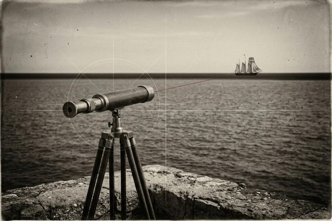
Proof the Earth Is Round: the flat earth arguments, tested
No single photograph proves a round Earth, because a photograph mixes geometry with lenses and weather. Independent measurements do: noon shadows change with latitude, the shadow on the Moon in every lunar eclipse is circular, Polaris sinks as you travel south, and long southern flights take the times a sphere predicts. Each argument below is run as a measurement, with the numbers you can change.
The flat earth arguments, one measurement each
Flat earth arguments are strongest when they are phrased as pictures and weakest when they are phrased as numbers. A picture of a distant skyline says the Earth cannot curve; a number says how much of a 400 metre tower should hide behind 90 kilometres of water and how much a layer of cooler air could lift back into view. The table lists the arguments met most often, the prediction a flat disc makes and the measurement that decides it.
A prediction only counts if it was written down before the result. For each row the flat disc is given its best case: a north-polar map with true distances from the centre, and a nearby lamp for the Sun. The round-Earth column uses one sphere for every row, with no adjustable parameter chosen after the fact.
| Argument | What the flat disc predicts | What is measured | Run it |
|---|---|---|---|
| Ships sink hull first | A ship shrinks smoothly with distance and can always be zoomed back into view. | From a 2 m eye height the water horizon lies about 5 km away, and the hidden height of a distant hull grows with the square of the distance. | Horizon distance tool → |
| Noon shadows differ between cities | A nearby Sun gives different angles at different places, but they fall on one lamp-height curve. | Eratosthenes’ 7.2° shadow difference over 800 km gives a 40,000 km circumference; a third site tests the curve. | Eratosthenes experiment → |
| The southern sky | One sky circles the north pole, so a southern observer sees the same northern stars. | Polaris stands as high as the latitude and sets below the horizon south of the equator; southern star trails circle a point above the south horizon. | Star trails tool → |
| Flights in the south | On the north-polar disc, Sydney to Santiago spans about 25,700 km, more than twice the sphere’s 11,300 km. | Scheduled southern flights take the times of the shorter great-circle distance, not the disc distance. | Flat earth map tool → |
| Day and night at the poles | One circling Sun lights the far north and far south of the disc in the same season. | Continuous daylight at the Arctic in June coincides with continuous night in Antarctica, and the two swap in December. | Day length calculator → |
| Earth does not move | Nothing turns beneath a swinging pendulum. | A Foucault pendulum’s swing plane turns by a rate that depends on latitude and reverses between hemispheres. | Foucault pendulum → |
| Water is always flat | A canal six miles long shows no curve between its markers. | Three equal-height markers across six miles of canal put the middle one about six feet above the chord. | Bedford Level experiment → |
Chicago skyline across Lake Michigan
A visible skyline is not the same as a visible shoreline. Test the height of a specific building feature against the observer’s height and the actual light path.
Keep the original observation attached
Joshua Nowicki · Grand Mere State Park · 30 April 2015
- Dated original
- Nowicki’s own gallery identifies Grand Mere State Park and 30 April 2015.
- Observation terrain
- The Michigan DNR describes dunes and Lake Michigan shoreline; the named park alone does not specify the camera’s elevation.
- Starting calculation
- 90 km separation, 2 m eye height and 400 m target are editable scenarios, not recovered photograph metadata.
- Needed for an exact image match
- Camera coordinates and height above that day’s lake level; identified building features; uncropped frame, time and vertical atmospheric profile.
Compare eye height, distance and light path
Change the sight-line scenario
These starting values define a comparison scenario. Replace the eye height, surface distance, target height and atmospheric assumption with your own paired observation.
Minimum radial height at the target needed to meet the limiting ray; zero before the observer’s horizon.
The entered target above the limiting ray; zero means the whole target is below that smooth-surface sightline.
Match one feature, not the word skyline
Select the roof, antenna tip or visible lower edge of one identified building. Those heights are different. A statement that “Chicago is visible” does not specify whether the water-level base, the upper storeys or a displaced refracted image is being seen.
The photographer’s named park contains shoreline and dunes. A location name cannot replace a measured eye height. Move the eye-height control through beach-level and elevated scenarios while retaining the same target and distance; compare hidden height with the chosen building feature.
Compare atmospheric scenarios with the same observation
Start with zero refraction, then compare an entered effective-radius coefficient. Keep the surface separation, eye and target fixed. The output shows how much of the target lies above a limiting ray, rather than treating tangent-plane drop as hidden building height.
A vertically changing refractivity profile may lift, stretch, invert or duplicate distant features. A single coefficient cannot reconstruct all of those effects. Use the layered-ray tool to compare gradients and collect temperature, pressure and humidity with height when repeating a lake observation.
What the dated image establishes
The original gallery anchors one photograph to an author, named park and date. It does not establish every geometric input in the starting scenario. Preserve the original frame and distinguish its capture date from the date on a repost or caption.
Compare repeated photographs from the same camera location and focal setting. An image that changes shape with weather is a different observation from a fixed straight-ray silhouette. Record which features move, whether the lake horizon is sharp and how the camera height was measured.
Lake Pontchartrain towers and causeway sight lines
The transmission line and the causeway are different observations. Compare dated positions and height datums before fitting a curve to a cropped image.
Keep the original observation attached
Lance Caraccioli · Three Lakeway Center · 5 January 2019 · causeway photograph

- FAA obstacle 22-001038
- 30° 17′ 38.00″ N, 90° 18′ 38.00″ W; transmission tower; 210 ft above ground, 211 ft above mean sea level; verified O status in the 27 September 2026 data cycle.
- FAA obstacle 22-000219
- 30° 17′ 49.00″ N, 90° 18′ 33.00″ W; another transmission tower; 210 ft above ground, 211 ft above mean sea level. Two catalogue records do not describe every tower in the crossing.
- A separate dated image
- Caraccioli’s own image record describes a 5 January 2019 causeway photograph with Sony a7R II and an 8-inch Schmidt–Cassegrain telescope, combined from 19 frames.
- Height datum
- AGL height is above the recorded ground reference, not automatically above the lake’s instantaneous water surface. Enter water level and the observation’s measured eye height in a common datum.
Compare eye height, distance and light path
Change the sight-line scenario
These starting values define a comparison scenario. Replace the eye height, surface distance, target height and atmospheric assumption with your own paired observation.
Minimum radial height at the target needed to meet the limiting ray; zero before the observer’s horizon.
The entered target above the limiting ray; zero means the whole target is below that smooth-surface sightline.
Project the two recorded tower tops
Enter one camera station to compare the FAA coordinates above. The starting station is a calculation scenario, not the station of a historical photograph. Elevation here is above mean sea level; the recorded tower tops are 64.3128 m AMSL.
| FAA tower | Surface range | Compass bearing | Spherical top angle | Level-plane top angle |
|---|---|---|---|---|
| 22-001038 | 10.489 km | 354.455° | 0.2932° | 0.3404° |
| 22-000219 | 10.816 km | 355.333° | 0.2815° | 0.3301° |
Both columns use the same recorded top elevations and surface ranges. The spherical column projects a straight ray relative to the camera’s local horizontal; the level-plane column places those ranges on a level plane. Neither fits atmospheric bending, lens distortion or intervening obstructions. Compare angular separation and elevation with identified tops in an uncropped frame. These two records are a subset of the crossing, and their 2026 elevations do not reconstruct every structure in a 2017 image.
Identify which line is being measured
The west-lake power line contains elevated transmission structures, while the highway causeway consists of many short spans and navigation passages. A photograph of one cannot supply the heights or alignment of the other. The two FAA tower coordinates shown here are catalogued obstacles; their height reference is separate from a photographed horizon.
Caraccioli’s causeway image has a dated original record. The image description and a surveyor’s camera record number the hotel floor differently, so use the actual surveyed camera height instead of converting a floor label into metres. This avoids silently treating a building-floor convention as an observation.
Perspective needs range as well as elevation
For a sequence of equal-height structures, every structure has its own distance and apparent vertical angle. Project those angles from one camera position. Drawing a line through the image’s tower tops without identifying ranges can confuse perspective with height differences.
The starting 20 km separation and 2 m eye height are scenarios. The 64.008 m target converts the catalogue’s 210 ft AGL; replace it with height above the measured water surface for an observation. A September 2026 catalogue entry is not proof that all dimensions of a 2017 photograph were identical.
Reconstruct a repeat observation
Record the camera station, water level and each matched tower or bridge feature at one date and time. Survey distances along the alignment rather than spacing markers evenly by their size in a photograph. Keep an uncropped frame so camera roll, lens projection and horizon placement can be checked.
Compare a straight-ray spherical prediction with an entered refraction scenario, then repeat at another eye height. The tower bases, tips and water horizon should be matched separately. Variable near-water temperature gradients need the layered-ray comparison rather than a universal refraction value.
How people measured Earth’s shape
A scale estimate from local observations
The traditional Eratosthenes account compares noon solar angles and the separation of two places. Converting ancient stadia into a modern kilometre figure involves uncertainty about the unit and reported baseline; distinguish that historical estimate from a newly measured experiment.
A sphere becomes an ellipsoid
Measuring meridian arcs at different latitudes revealed that a single spherical radius was insufficient for precise surveying. An oblate reference ellipsoid captures the systematic equatorial and polar difference. The geoid describes the additional gravity-related shape.
The Columbus story does not establish a medieval flat consensus
The historical dispute over an Atlantic crossing included the size of Earth and the distance to Asia. A claim that educated Europeans universally expected a flat edge confuses those disagreements with a different proposition. Follow specific texts and measurements rather than treating one popular story as a whole era.
The modern flat-Earth movement in its own archive
Samuel Shenton’s correspondence uses a letterhead for the International Flat Earth Research Society, dated to its 1956 founding and based in Dover, England. A 23 February 1967 letter discusses preparing posters for a science fair and appearances on television and radio. This is evidence of an organised modern campaign and its communication methods, rather than evidence about Earth’s geometry.
The society’s library preserves Shenton’s letters alongside Charles K. Johnson correspondence from 1971 and later newsletters. These named records let a reader distinguish the modern movement from earlier writings such as William Carpenter’s 1885 pamphlet and Samuel Rowbotham’s nineteenth-century arguments. Assess a proposed measurement separately from the group that circulated it.
Compare explanations without arguing about a label
Start with a precise claim
Ask which distance, angle, direction or contact time the claim predicts. “The world looks flat” is not yet a numerical prediction; a horizon angle at one specified camera height is. Agree the units and the reference direction before changing the inputs.
Allow the same test to challenge both models
Write both results before observing. Avoid granting one explanation adjustable parameters after the measurement while holding the other fixed. If both fit within uncertainty, choose another observation with greater separation. The three-shadow tool illustrates how an additional site can test the shape of a relationship.
Make the next step practical
Keep a source file or raw reading both people can inspect. Ask what each would expect if their explanation were wrong. Let an unresolved observation remain open instead of turning it into a contest over intelligence or identity.